Fast MCS

Overview
Project contributions
Areas of improvement

Overview

This project provides a fast updating implementation of the Model Confidence Set (MCS) algorithm (Hansen et al., 2011). It is actually an old project that has evolved over the years. Its origin lies in when I was working on my application of the MIC to agent-based model selection on financial markets (Barde, 2016). Because the MIC is essentially a noisy measurement of the AIC for simulation models, one needs to account for the fact that differences in model rankings may not be statistically significant. A colleague helpfully suggested the MCS approach, which at the time was relatively new, which was helpful. However, with the 513 specifications used in the analysis, it took a looooong time to run, and attempts at larger collections rapidly exhausted the 8GB of RAM on my desktop (In those days, that was considered a lot).

This prompted me to investigate the scaling characteristics of the MCS approach, and see if it was possible to improve on this. The intuition laid out below arrived quickly, but the proof of equivalence took much longer (embarrassingly so I’m afraid to say). Details of all this, in particular the proofs is provided in (Barde, 2024). The MCS approach uses losses $\mathcal{L}$ for a collection of $M$ models, and iteratively identifies the worst performing model and eliminates it from the collection if the performance is significantly worse. This process continues until the null of equal predictive ability cannot be rejected for the candidate model, and the surviving models comprise the MCS. This process, referred to as the elimination implementation, requires an appropriate elimination statistic to identify the candidate model and a suitable bootstrap for the P-values, however it is incredibly intuitive.

The MCS procedure requires an $N \times M$ set of losses $L$, in order to calculate the relative loss $d_{i,j,n} \equiv L_{n,i} - L_{n,j}$ of model $i$ relative to model $j$. These are used to calculate the following set of t-statistics under the null hypothesis that all expected mean pairwise deviations are zero-valued, i.e. $H_0: E[\bar d_{i,j}]=0$:

\[t_{i,j} = \frac{ \bar d_{i,j} }{ \hat \sigma_b \left( \delta_{i,j,b} \right)} \tag{1}\]

The standard deviation of the sample average $\bar d_{i,j}$ is estimated using a bootstrap, where a set of $N \times B$ bootstrap indices $\mathcal{B}$ allows us to generate an $N \times M \times B$ array of resampled loss matrices $\mathcal{L}$. This is used to calculate resampled pairwise deviations:

\[\delta_{i,j,b} = \frac{1}{N} \sum_n \left( \mathcal{L} _{n,i,b} - \mathcal{L} _{n,j,b} \right) \tag{2}\]

Under the range (R) rule - which is the one used as the basis of the fastMCS procedure, the worst-performing model, also the candidate for elimination in any iteration, is the one having the largest pairwise t-statistic $t_{i,j}$, i.e. the one that has the highest average normalized loss relative to any other model still in the collection.

\begin{align} e_k = \arg \max_{i \in \mathcal{M}} \max_{j \in \mathcal{M}} \left(t_{i,j}\right) & & T_{e_k} = \max_{i \in \mathcal{M}} \max_{j \in \mathcal{M}}|t_{i,j}| \tag{3} \end{align}

The distribution of this elimination statistic, which is used to test $H_0$ against the alternate hypothesis $H_A: E[\bar d_{i,j}] \ne 0$, is obtained using bootstrapped pairwise deviations:

\[\tau_{i,j,b} = \frac{ \delta_{i,j,b} - \bar d_{i,j}}{ \hat \sigma_b \left( \delta_{i,j,b} \right)} \tag{4}\]

These are used to generate the bootstrapped elimination statistics and associated bootstrapped p-values, where $I(\dots)$ is the Boolean indicator function:

\begin{align} \label{eq:p-value} \mathcal{T}_ {e_k,b} = \max_{i \in \mathcal{M}} \max_{j \in \mathcal{M}} |\tau_{i,j,b}| & & P_{e_k} = \max\left(P_{e_{k-1}},\frac{1}{B}\sum\nolimits_b {I\left( \mathcal{T}_ {e_k,b} \ge T_{e_k} \right)}\right) \tag{5} \end{align}

The following algorithm summarizes the MCS iterative elimination procedure.

\begin{algorithm}
\caption{Elimination MCS}
\begin{algorithmic}
\REQUIRE $$L$$: an $$N$$ by $$M$$ matrix of losses
\REQUIRE $$Bi$$: an $$N$$ by $$B$$ matrix of bootstrap indexes
\PROCEDURE{Eliminate}{$$L, Bi$$}
  \STATE $$t <= $$ Calculate matrix of t-statistics with (1)
  \STATE $$tau <= $$ Calculate matrices of bootstrapped statistics with (4)
  \FOR{$$k = 0$$ \TO $$M$$}
    \STATE $$e, T <= $$ Find worst model with elimination rule (3)
    \STATE $$Tb <= $$ Find bootstrapped statistics with (5)
    \STATE $$P <= $$ Calculate bootstrapped p-value with (5)
    \STATE Remove row/column $$e$$ from $$t$$ and $$tau$$
  \ENDFOR
\ENDPROCEDURE
\RETURN $$T$$, $$P$$
\end{algorithmic}
\end{algorithm}

Given a candidate collection of $M$ models, the elimination implementation has a $\mathcal{O}(M^3)$ time complexity and a $\mathcal{O}(M^2)$ memory requirement. The former comes from the fact that the model will have $\mathcal{O}(M)$ iterations, each requiring finding the maximum of an $M \times M$ matrix. The latter comes from having to store $B$ bootstrapped versions of the original $M \times M$ elimination statistics.

The fastMCS updating implementation reduces this down to a $\mathcal{O}(M^2)$ time complexity and a $\mathcal{O}(M)$ memory requirement. This is done by flipping the processing sequence, i.e. the algorithm starts with a collection of 1 model, successively adds models (rather than removing them), updating the existing rankings and p-values. Computationally, this means that each iteration now only processes vectors, rather than matrices, which explains the reduction of all requirements (time and memory) by one polynomial order. Given a model $m$ added to an existing collection, the vector of elimination statistics (and thererefore the elimination sequence) of the exisiting collection $T_k$, can be updated using the following rules, where $\mathcal{E}_ {m}^{-}$ and $\mathcal{E}_ {m}^{+}$ denote the set of models eliminated respectively before and after $m$:

\[\left\{ \begin{align} T_k & = T'_ k & \qquad \forall \enspace k \in \mathcal{E} \_m^+ \\ T_m & = \mathop {\max }\limits_i \left( { t_{m,i} } \right) & \qquad \forall \enspace i \in \mathcal{M}' \\ T_k & = \max \left( {T'_ k ,t_{k,m} } \right) & \qquad \forall \enspace k \in \mathcal{E} _m^- \\ \end{align} \right. \tag{6}\]

The bootstrapped t-statistics of the previous collection, $\mathcal{T}'_ {k,b}$ are updated using a similar set of rules:

\[\left\{ \begin{align} \mathcal{T}_ {k,b} & = \mathcal{T}'_ {k,b} & \qquad \forall \enspace k \in \mathcal{E} \_m^+ \\ \mathcal{T}_ {m,b} & = \max \left(\mathcal{T}'_ {m^+,b} \, , \, \mathop {\max }\limits_i |\tau_{m,i,b}| \right) & \qquad i \in \mathcal{E} \_{m}^{+} \\ \mathcal{T}_ {k,b} & = \max \left(\mathcal{T}'_ {k,b} \, , \, \mathop {\max }\limits_i |\tau_{m,i,b}| \right) & \qquad \forall \enspace k \in \mathcal{E}_ m^-, i\in\mathcal{E} _k^+ \\ \end{align}\right. \tag{7}\]

Note the updating rules (6) can be shown to work for all models $m$ that are not in the set of superior models $\mathcal{M}$. The updating rules (7) only actually work under the restrictive (and unrealistic) assumptions that when a model $m$ is added it does not disturb the rankings of worse-ranked models. Nevertheless, this is enough to establish that the updating algorithm 2 will provide identical output to the elimination algorithm 1 for all models not in the superior set $\mathcal{M}$. Details of why this is are provided in the paper, however this provides intuition as to why a 2-pass approach is used: The first pass generates the elimination statistics, and this the model rankings. In the second pass, models are processed in reverse elimination order to obtain the p-values. Given this, the two-pass version of the fast updating algorithm is outlined below:

\begin{algorithm}
\caption{Two-pass Fast updating MCS}
\begin{algorithmic}
\REQUIRE $$L$$: an $$N$$ by $$M$$ matrix of losses
\REQUIRE $$Bi$$: an $$N$$ by $$B$$ matrix of bootstrap indexes
\PROCEDURE{ModelRankings}{$$L$$}
  \STATE $$t <= $$ Calculate vector of t-statistics with (1)
  \STATE $$T <= $$ Update model rankings with (6)
\ENDPROCEDURE
\STATE $$e <= $$ Sort models by ascending value of $$T$$
\PROCEDURE{Pvalues}{$$L,Bi,e$$}
  \FOR{$$i = 0$$ \TO $$M$$}
    \STATE $$m <= e[i]$$
    \STATE $$tau <= $$ Calculate vectors of bootstrapped statistics with (4)
    \STATE $$Tb <= $$ Update bootstrapped statistics with (7)
    \STATE $$P <= $$ Calculate bootstrapped p-value with (4)
  \ENDFOR
\ENDPROCEDURE
\RETURN $$T$$, $$P$$
\end{algorithmic}
\end{algorithm}

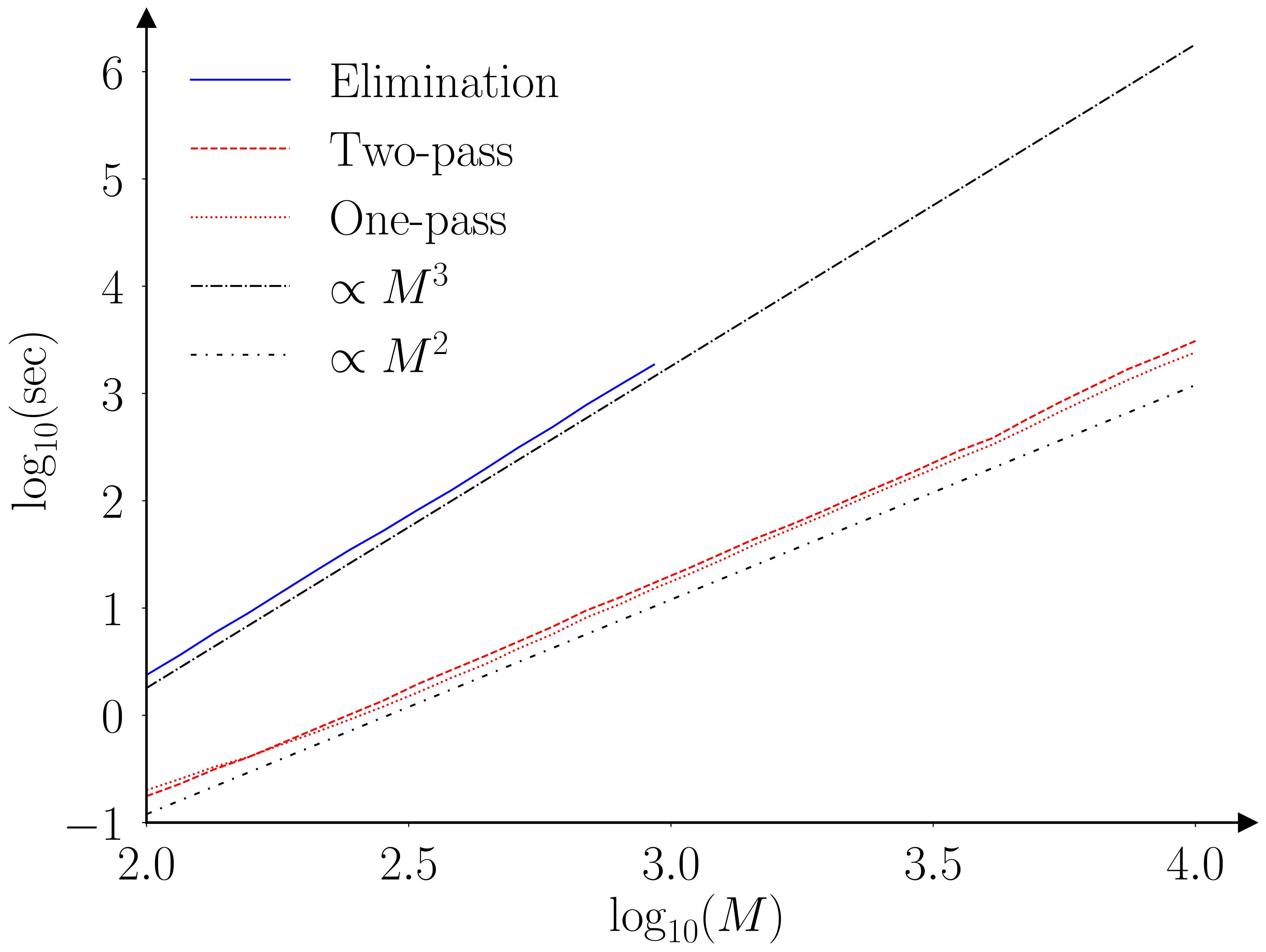
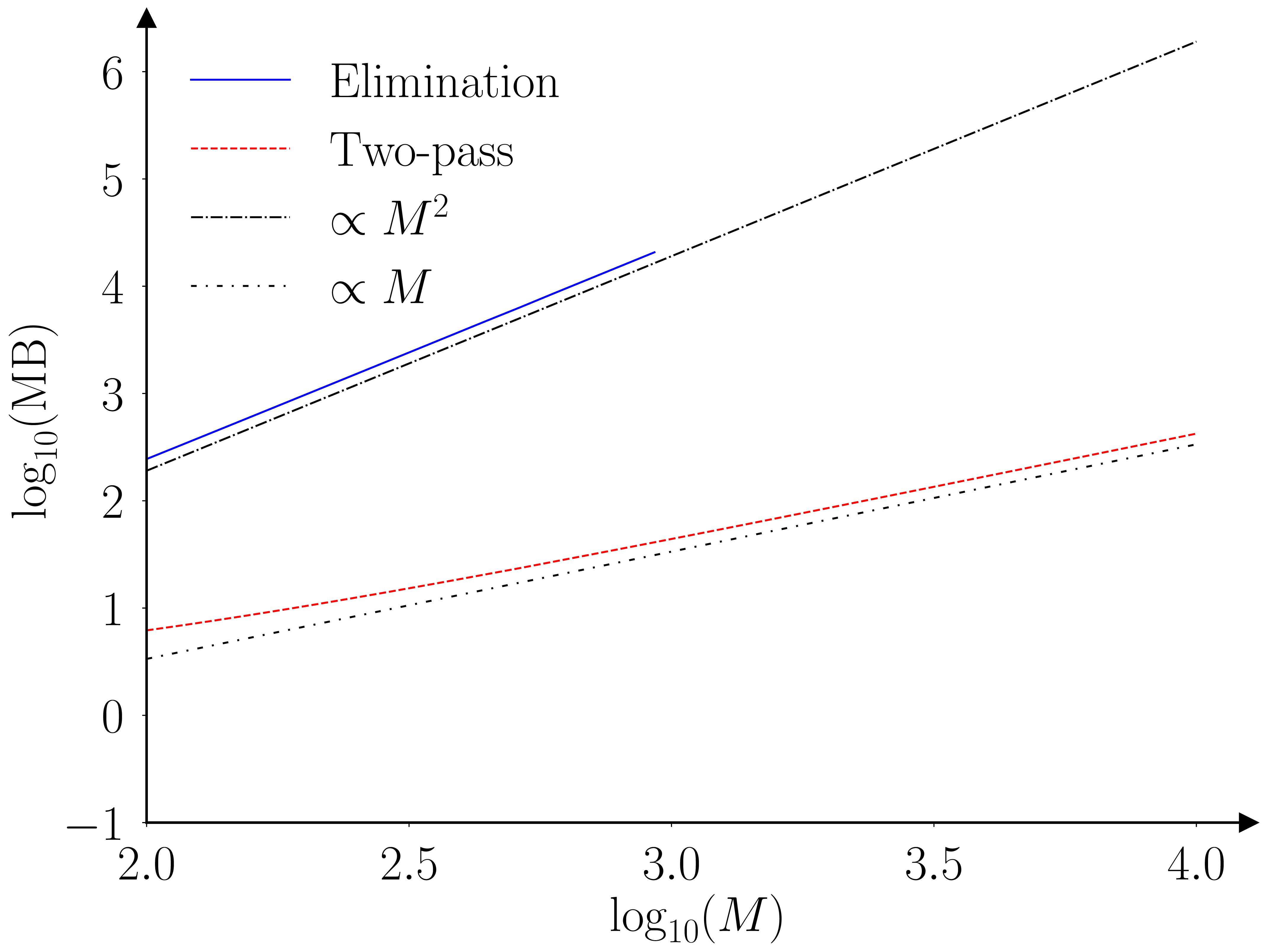
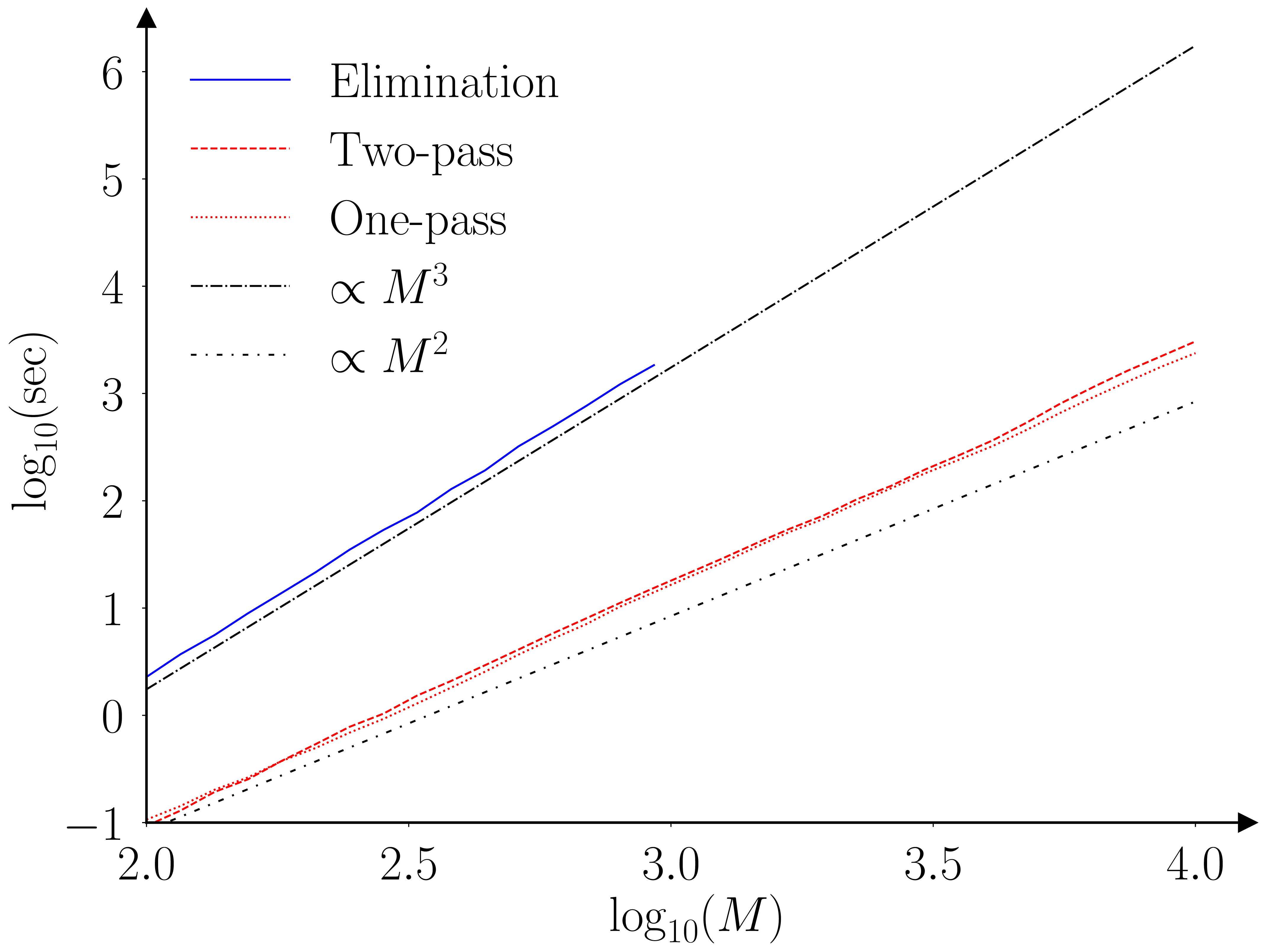
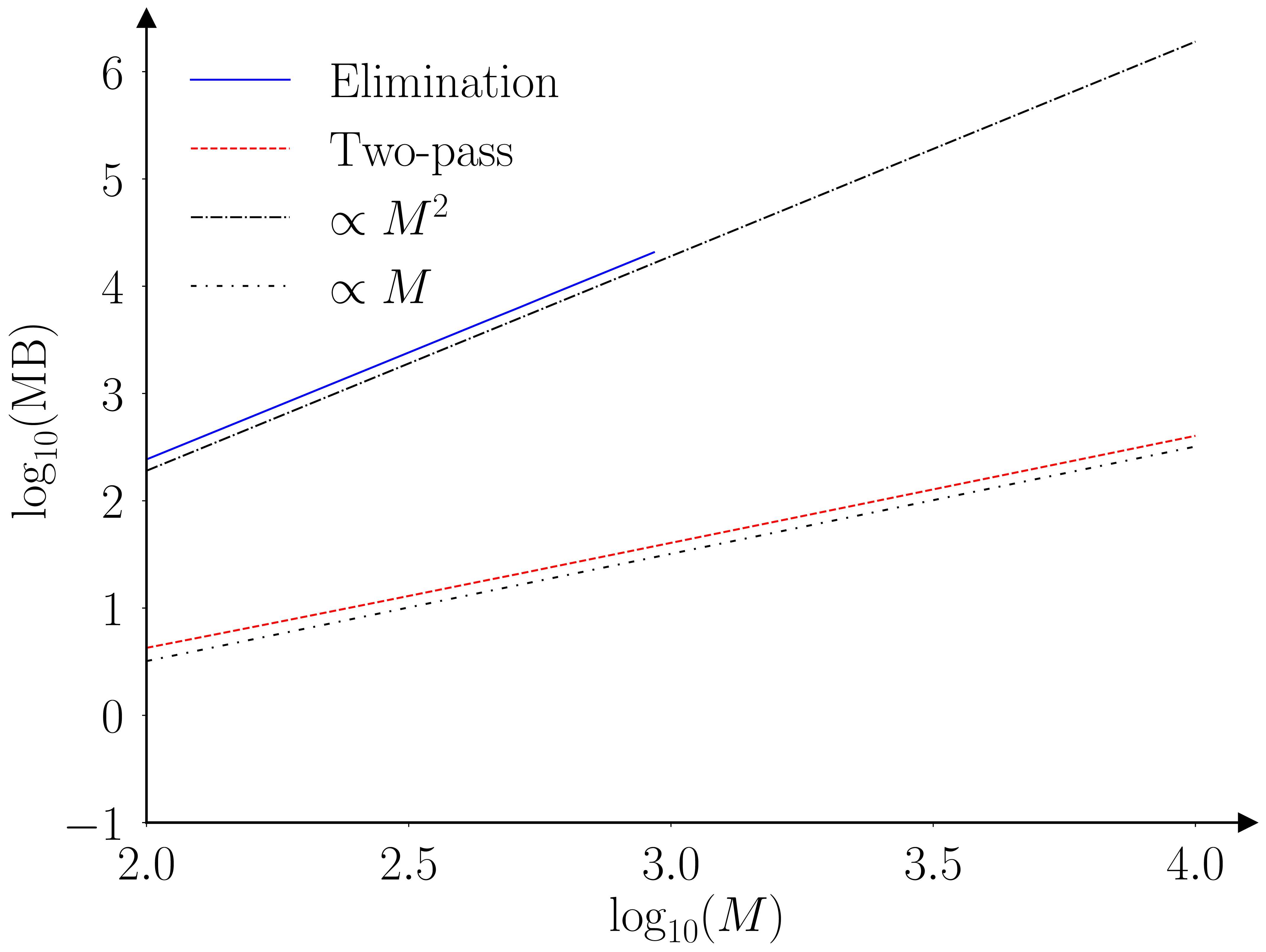
The paper (Barde, 2024) runs a benchmarking exercise using the original Monte-Carlo testing exercise of (Hansen et al., 2011), the results of which are provided in the figures below.

These plots show the time (left plot) and memory (right plot) benchmarking exercises in log units for an empirical sample of N=250 observations. The trajectories confirm the cubic time complexity and quadratic memory requirement for the elimination algorithm. The equivalent requirements for the updating algorithm are quadratic and linear respectively.

The two algorithms (elimination and fastMCS) are proven to provide equivalent output, however this is an ‘almost surely as $N \to \infty$’ result. I’m not that worried, as the practical rate of convergence is likely to be very fast, as the elimination statistic is an order statistic, due to the fact we are looking at a ‘maximum’. To be safe I ran a second exercise with $N=30$ to check for any deviations. The two algorithms still provide identical output, even for this small sample size.

These are equivalent benchmarking plots for the N=30 case. Crucially, even for such a small evaluation sample, in every case the model rankings and p-values outputed by the updating algorithm exactly match those of the elimination algorithm.

The practical implication of these improved scaling characteristics are illustrated by the following table. This extrapolate the benchmarking results obtained for the elimination MCS to larger collections. The last row indicates that establishing the MCS of a collection of 10,000 models would require 579 hours (~24 days) and require 2.4 TB of RAM in doing so. The fastMCS algorithm can achieve the same task in 40 minutes with 423 MB.

	Elimination		Two-pass
	Time (sec)	Memory (MB)	Time (sec)	Memory (MB)
M = 500	295	6,017	3	23
M = 1,000	2,318	24,055	11	44
M = 2,000	17,735	96,219	67	86
M = 5,000	265,314	601,399	557	212
M = 10,000	2,084,924	2,405,669	2,441	423

Benchmarking performance in 'human' units for collections of size M. The performance gains are huge, especially for larger collections.

Project contributions

What bits does this project reach that others don’t?

Well, clearly, the performance gains on large collections are valuable in themselves, as it unlocks types of large-scale forecasting evaluations that were not tractable before. Combine this with today’s big data world and incentives to provide better forecasts (of financial volatility, of commodity prices, of the weather, etc.) and it is not hard to see potential benefits. Of course, most of the academic literature using the MCS tends to use small collections to test novel methods against a handful of benchmarks, in such cases the elimination MCS will be perfectly adequate.
A second benefit, even for small comparisons, is that by updating the MCS as models are added, rather than shrinking the MCS as models are eliminated, allows for a comparison exercise to be updated ex-post. Suppose you have access to an HPC service and pay the cost involved in running an M=10,000 collection, as in the table above. 24 days later, you have your MCS. If at that point you realise that you forgot to include 100 models from an obscure corner of the forecasting literature, you have no choice than to re-run the whole thing. With fastMCS, you can just update your MCS with these 100 models at a fraction of the compute cost. This re-introduces the possibility of collaborative research in the spirit of (White, 2000), where researchers post their model losses, bootstrap indices and MCS results (elimination statistics and P-values) so that subsequent researchers can build on them at a later date.

Areas of improvement

Things I’m not that happy about right now.

A first consideration, as mentioned above, is that most uses of the MCS have small collections (less than 10 models), where this performance improvement will not matter. So fastMCS might not necessarily displace the elimination approach in practice. I’m fine with that personally!
Right now, this works for the ‘R’ (range) elimination rule only. I’ve not looked at the other rule proposed by (Hansen et al., 2011), the ‘max’ rule, where candidates for elimination are selected based on their deviation from average performance in the collection. So this means that fastMCS is not currently as flexible as the elimination approach. I suspect that this is harder, as the average needs to be re-calculated in between iterations. It should be possible to re-calculate the average and the elimination statistics of existing models when a model is added, but whether the same can be done for the bootstrapped statistics is an open question. However, this is an interesting area for other research.

The paper proposes a new algorithm for finding the confidence set of a collection of forecasts or prediction models. Existing numerical implementations use an elimination approach, where one starts with the full collection of models and successively eliminates the worst performing until the null of equal predictive ability is no longer rejected at a given confidence level. The intuition behind the proposed implementation lies in reversing the process, i.e. starting with a collection of two models and updating both the model rankings and p-values as models are successively added to the collection. The first benefit of this approach is a reduction of one polynomial order in both the time complexity and memory cost of finding the confidence set of a collection of M models, falling respectively from O(M^3) to O(M^2) and from O(M^2) to O(M). The second key benefit is that it allows for further models to be added at a later point in time, thus enabling collaborative efforts using the model confidence set procedure. We prove that this implementation is equivalent to the elimination approach and demonstrate the improved performance on a multivariate GARCH collection consisting of 4800 models.

The present paper tests a new model comparison methodology by comparing multiple calibrations of three agent-based models of financial markets on the daily returns of 24 stock market indices and exchange rate series. The models chosen for this empirical application are the herding model of Gilli and Winker (2003), its asymmetric version by Alfarano et al. (2005) and the more recent model by Franke and Westerhoff (2011), which all share a common lineage to the herding model introduced by Kirman (1993). In addition, standard ARCH processes are included for each financial series to provide a benchmark for the explanatory power of the models. The methodology provides a consistent and statistically significant ranking of the three models. More importantly, it also reveals that the best performing model, Franke and Westerhoff, is generally not distinguishable from an ARCH-type process, suggesting their explanatory power on the data is similar.

Table of contents

Overview

Project contributions

What bits does this project reach that others don’t?

Areas of improvement

Things I’m not that happy about right now.

References

2024

2016

2011

2000

References

2026
2016
- Direct comparison of agent-based models of herding in financial marketsJournal of Economic Dynamics and Control, 2016
2011
- The Model Confidence SetEconometrica, 2011
2000
- A Reality Check For Data SnoopingEconometrica, 2000