BEGRS

Table of contents

• Overview
• Project contributions
• Areas of improvement

Overview

This was one of my COVID projects. Like many, I found myself having more time than expected, stuck in closed quarters, and I needed something to channel the cabin fever… So I started scratching my head over the problem of estimating the large, computationally burdensome agent-based models that my colleagues had developed over the years. There are plenty of indirect inference methods out there for estimating the deep parameters of simulation models, but these often rely on in-the-loop or open-ended simulations of the model. With large agent-based models that take minutes to generate a single simulation run, these methods just don’t scale… I needed to find a way to do more with less.

The full details for this are provided in (Barde, 2024), however, as a quick overview, the methodology uses a Gaussian process as a surrogate model for the one-step ahead prediction of the model given an observed state and some model parameters.

In many ways, this first pass at the problem is kind of low-tech: no Bayesian learning of the parameter space is carried out to acquire samples, no empirical data is used to generate deviations. All this is designed to reduce the compute burden involved in simulating the underling model. In practice, in order to keep the problem computationally tractable, the GP is trained using the variational methods of (Hensman et al., 2015) using the GPpytorch toolbox of (Gardner et al., 2018) to provide GPU acceleration.

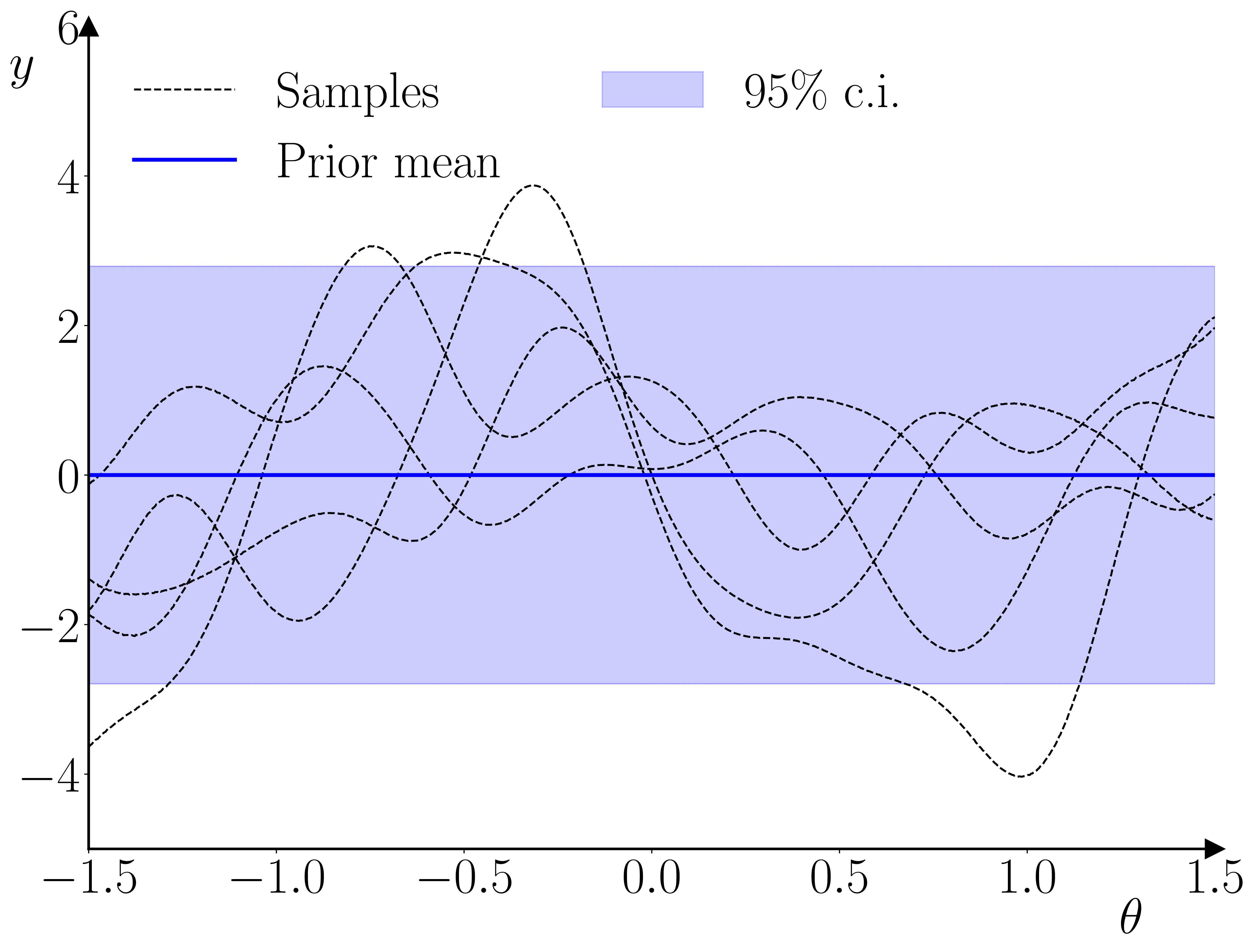
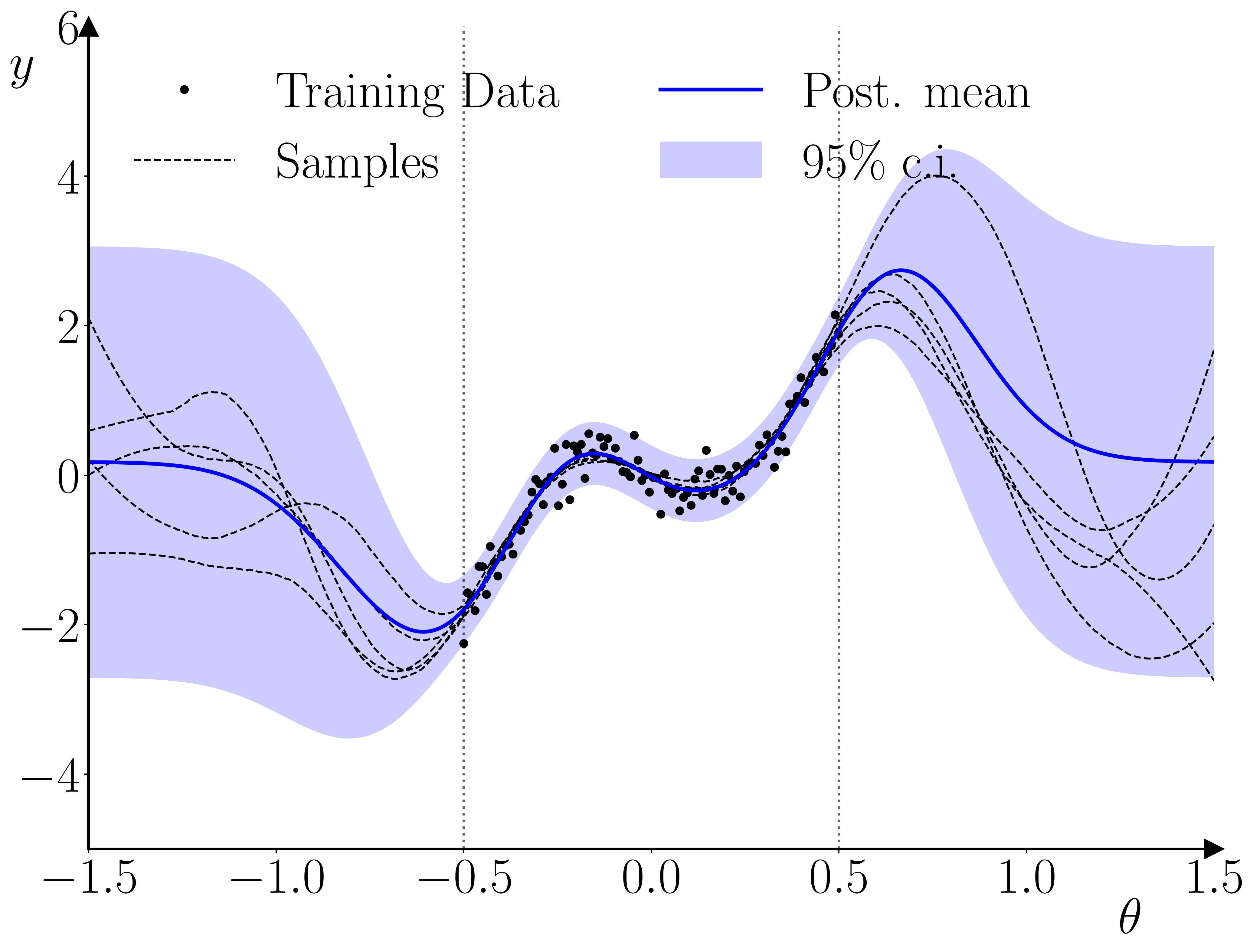
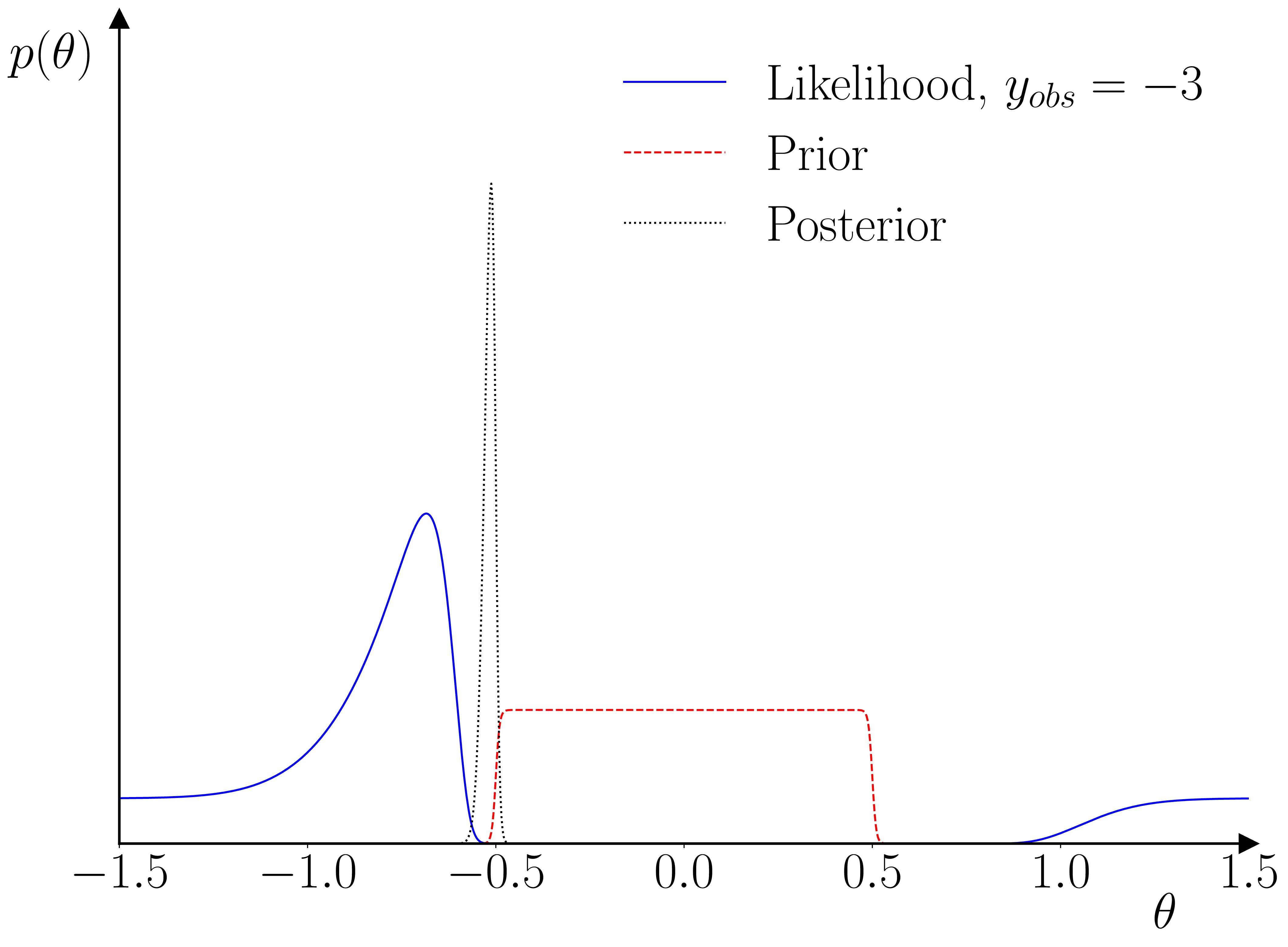
Once the GP surrogate is trained, it can be used in a second stage to provide a surrogate likelihood in a standard Bayesian estimation for an observation \(y_t\), given \(y_{t-1}\) and a parameter vector \(\theta\). The only requirement the methodology has relative to standard Bayesian methods is that the prior on the parameter vector must constrain the parameter space to the hypercube within which the training parameter samples were drawn. The reason for this requirement is illustrated below.

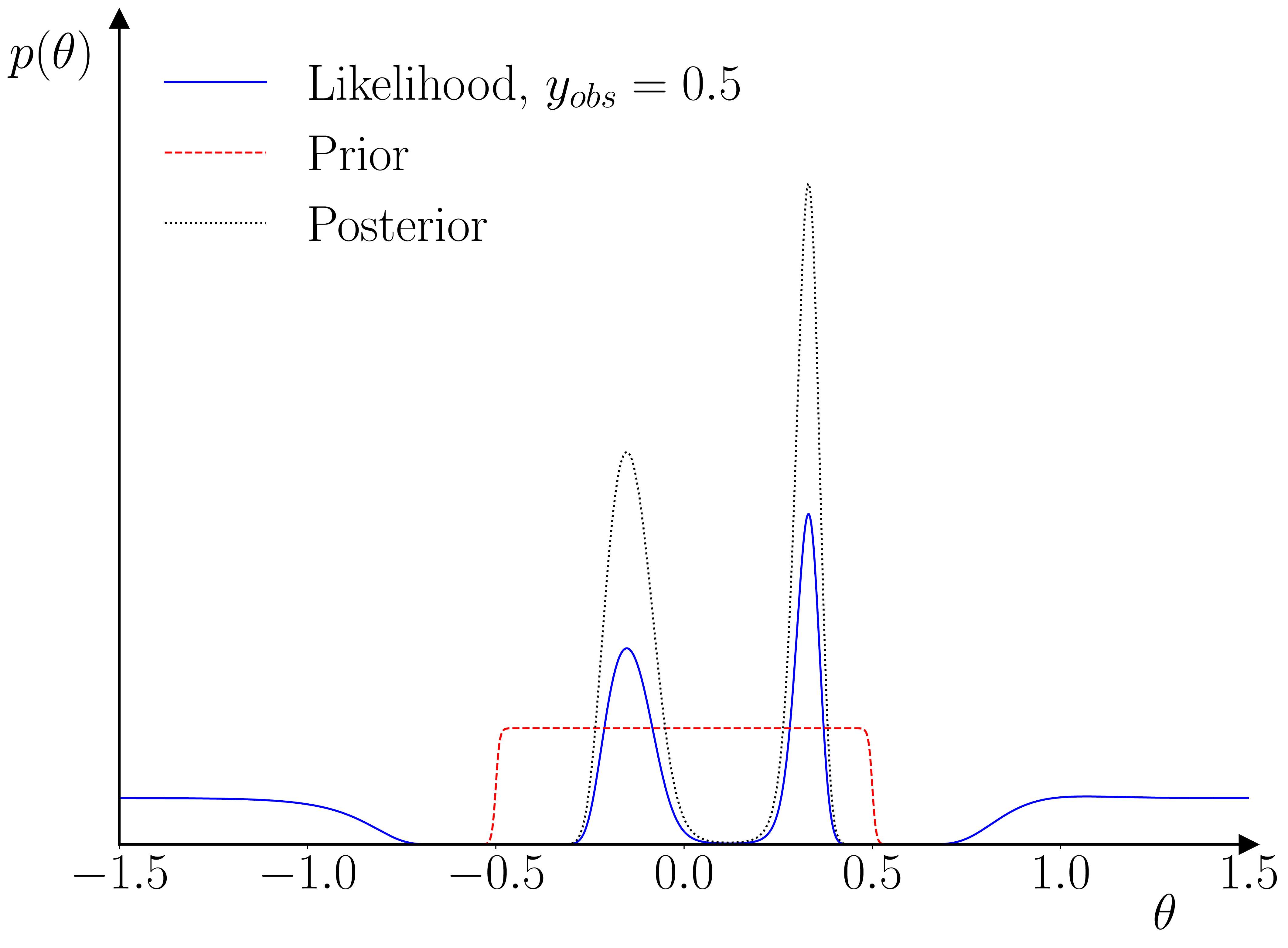
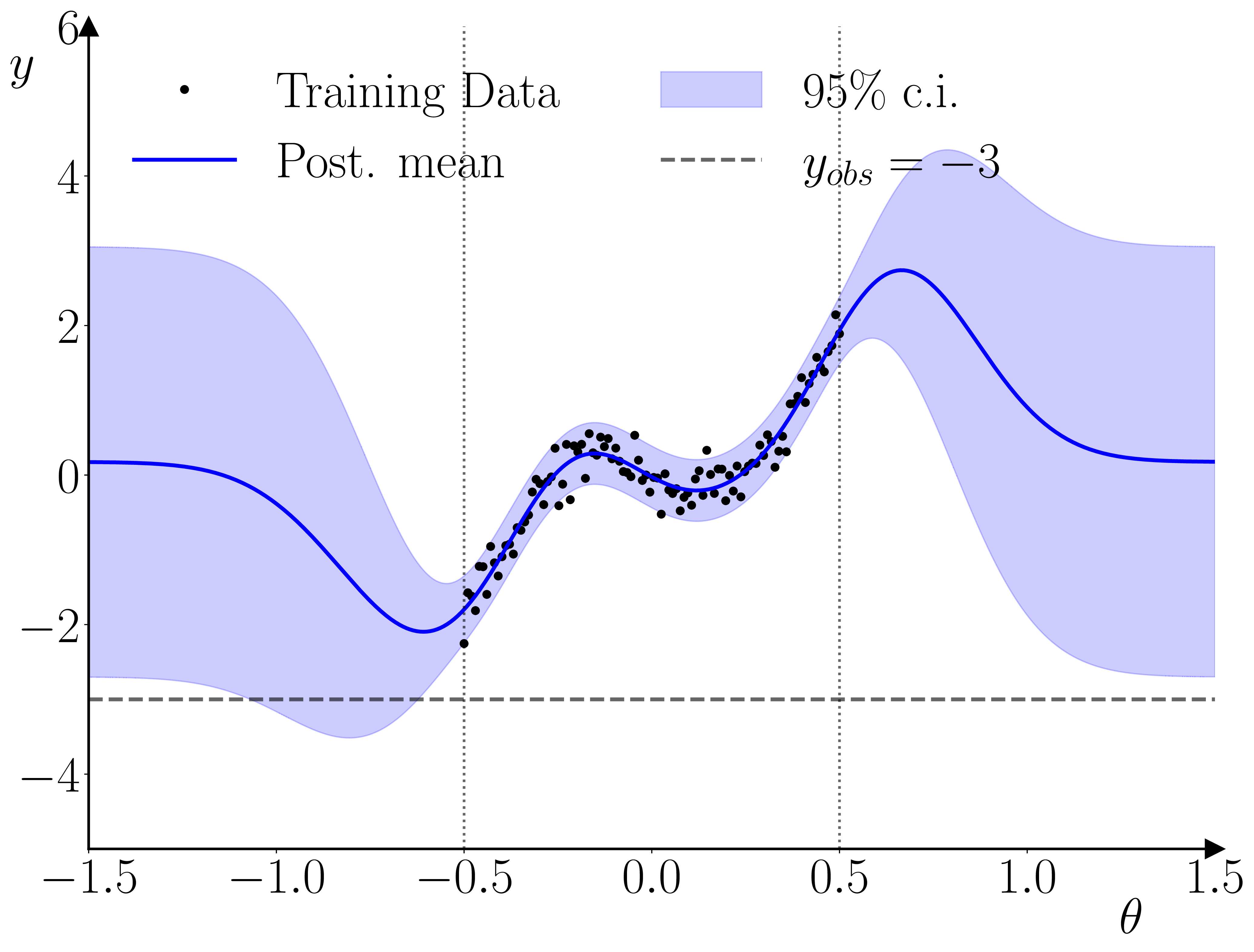
One neat thing that I hadn’t initially realized is that this setup actually provides a kind of ‘fault-detection’ for the training data used in the training of the GP surrogate. As illustrated below, if the empirical observation is inconsistent with the range used in the training, then the GP prior will dominate the GP posterior, and the likelihood’s peak(s) will occur outside of the parameter range used for the training data. The parameter prior will pinch this off, resulting in a quasi-degenerate parameter posterior on the boundary.

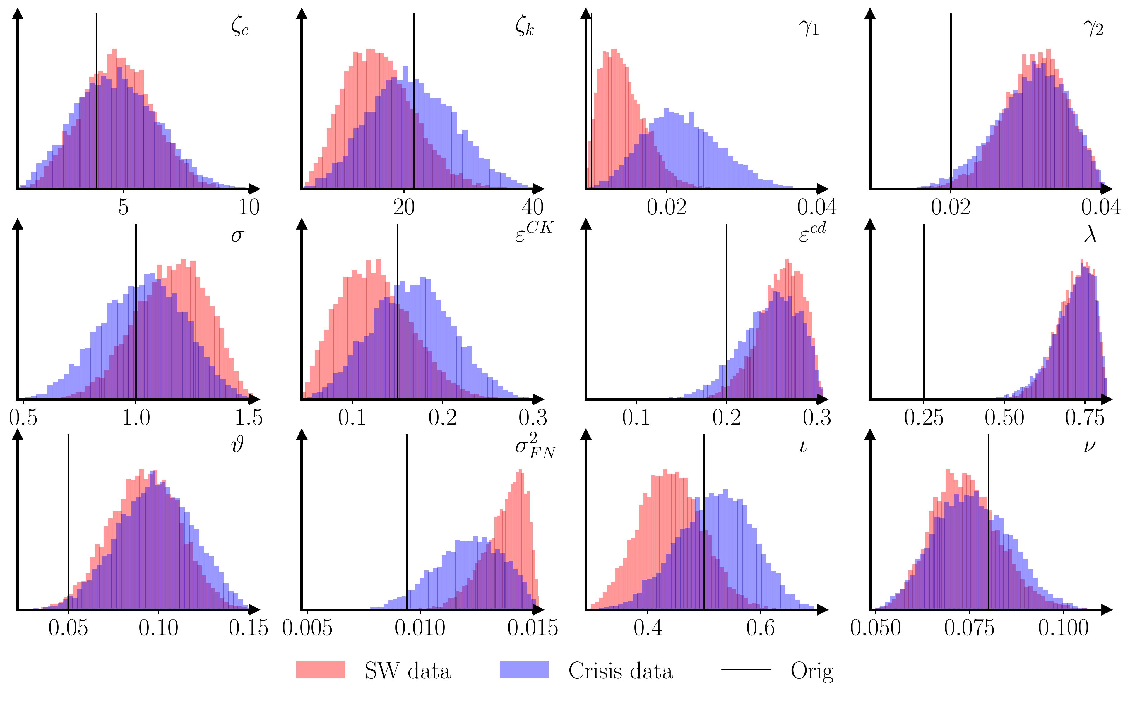
As a practical example, I’ve applied the methodology to the (Caiani et al., 2016) model. It can take the original model 40 minutes to produce a usable 200-300 long macro time series, so in-the-loop simulation is out of the question. 1000 simulations of 200 observations each, using parametrizations drawn from a Sobol sequence, are enough to produce a decent set of estimates for the 12 free parameters.

Project contributions

What bits does this project reach that others don’t?

The methodology as implemented has several nice characteristics:

• GP gradients are easy to compute, so gradient-based methods, such as BFGS for finding the mode of the posterior or Hamiltonian MCMC for drawing posterior samples, can be implemented out-of-the-box.
• Because the second stage parameter estimation (given the GP surrogate) is a standard Bayesian framework, a full Bayesian workflow can be followed, including posterior checks, for example (Cook et al., 2006), or (Talts et al., 2018).
• Finally, that the methodology seems to perform well with limited training data, so given all the compromises made on the surrogate model (see next section!) it’s ‘mission accomplished’ for the central aim.
• This is improved by the fact that the surrogate does not require retraining before estimation on different datasets. For instance, the same surrogate is used in the US empirical estimation above.

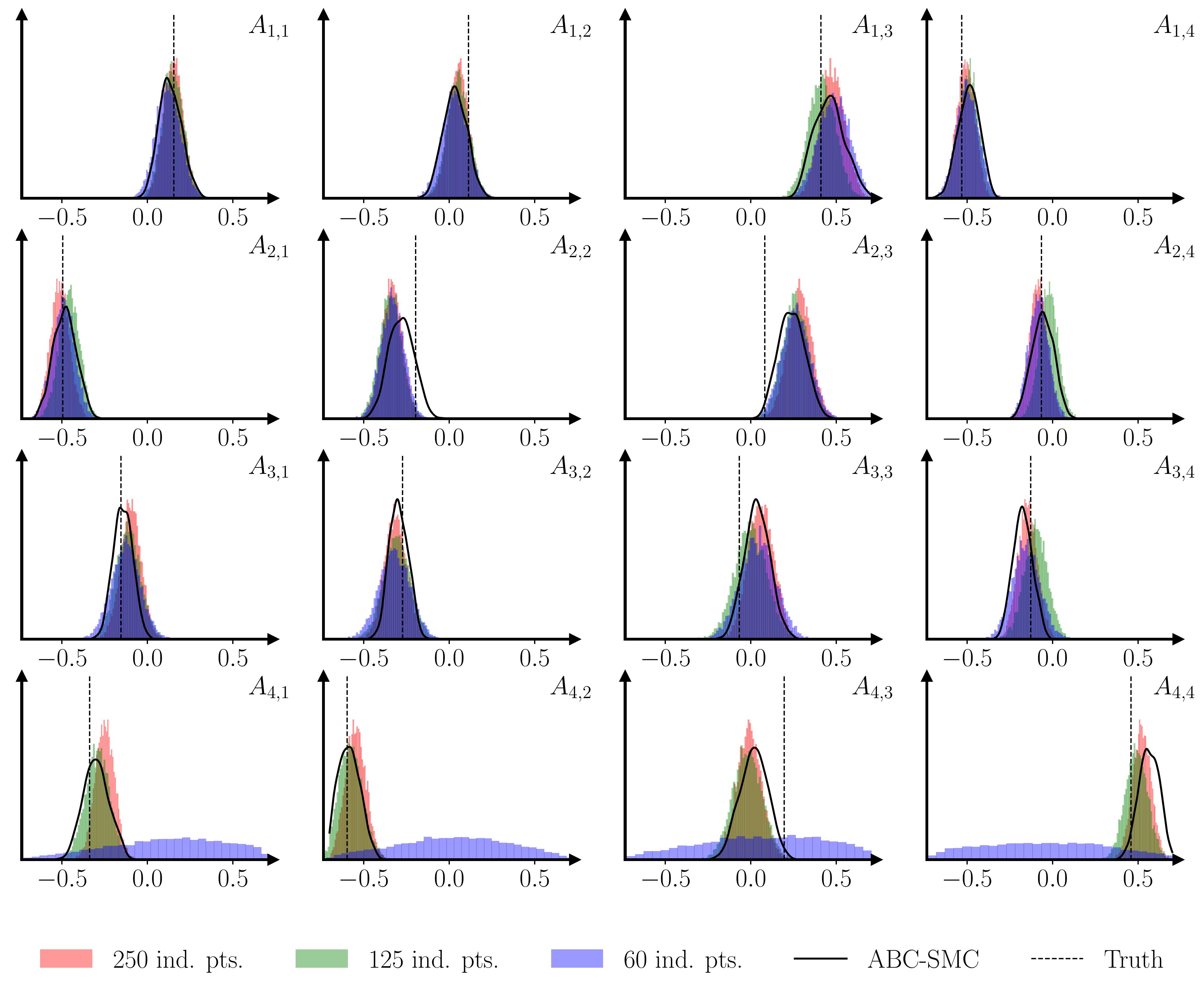
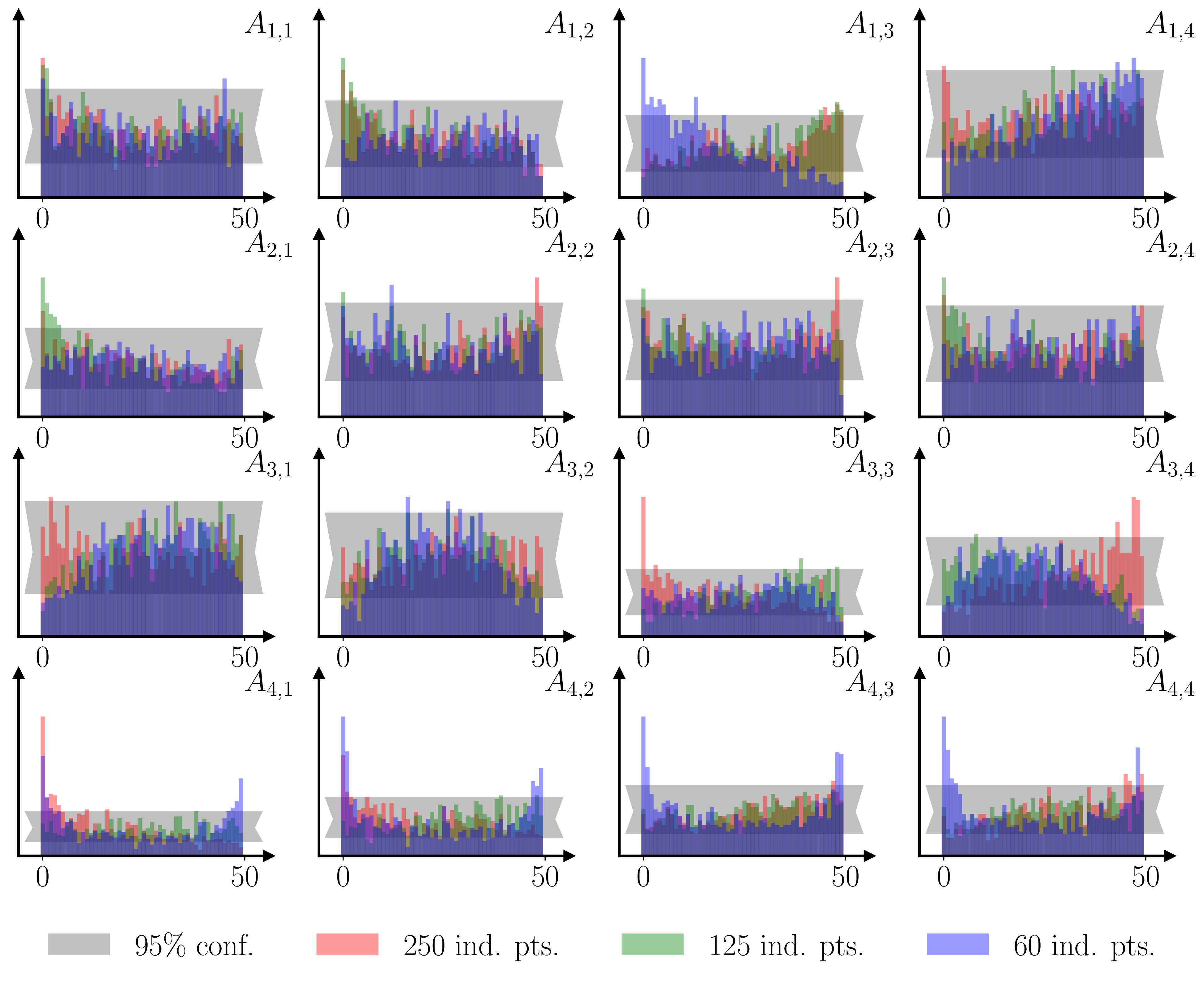
As a sanity check, and an illustration of the last two points, I ran a simple Monte Carlo example, training a GP surrogate using 1000 simulations of VAR(1) models with 4 variables and 200 observations, where the 16 parameters of the autoregressive matrix were drawn from Sobol sequences. Both a parameter recovery exercise and a Simulated Bayesian Computing posterior check (Talts et al., 2018) show that the methodology performs well.

Areas of improvement

Things I’m not that happy about right now.

Well, a lot of nice things were sacrificed as part of the drive to make a simple model that generalises well with minimal training data.

• The Vecchia approximation (i.e. one-step ahead prediction_) might not be appropriate for models with highly non-linear responses or long memory. The VAR(1) case is fine, but SBC analyses of longer memory models reveal that the BEGRS posterior is often too narrow.
• Similarly, the Sobol sampling scheme used in my current BEGRS applications will struggle with discontinuities in the responses. This will slow convergence with respect to the number of training samples, requiring further training samples. I aim to investigate this using either deep gaussian learning, or adaptive sampling methods (e.g. Bayesian sampling based on prediction entropy).

References

2024
- Bayesian estimation of large-scale simulation models with Gaussian process regression surrogatesComputational Statistics & Data Analysis, 2024
2018
- Gpytorch: Blackbox matrix-matrix gaussian process inference with gpu accelerationAdvances in neural information processing systems, 2018
- Validating Bayesian inference algorithms with simulation-based calibrationarXiv preprint arXiv:1804.06788, 2018
2016
- Agent based-stock flow consistent macroeconomics: Towards a benchmark modelJournal of Economic Dynamics and Control, 2016
2015
- Scalable variational Gaussian process classificationIn Artificial Intelligence and Statistics, 2015
2006
- Validation of software for Bayesian models using posterior quantilesJournal of Computational and Graphical Statistics, 2006